

Import CSV data into Python
We'll demonstrate that you can go from downloading a dataset to getting valuable insights from it in just a few minutes. You can obtain a high-quality Car Dataset from Germany in CSV with more than 45.000 records.
Prerequisites
For the code to work, you will need python3 installed. Some systems have it pre-installed. After that, install all the necessary libraries by running pip install.
pip install pandas matplotlib squarify seaborn
First, import the data from the dataset file. Create a python file or open a console in the folder containing the CSV file. Pandas comes with a handy function read_csv to create a DataFrame from a file path or buffer.
Import the lib and call that function with your local route to the dataset file. In our case, it is a relative path. It will generate a variable called cars that will contain all the data from the file.
import pandas as pd

cars = pd.read_csv('./germany-cars-zenrows.csv')
Exploratory Data Analysis
Once we have the data accessible, we can start using it in our code. The problem is, we probably don't know anything about its content or even structure.
This command will show a sample with 20 rows. You can see below a summarized example.
cars.sample(frac=1).head(n=20)
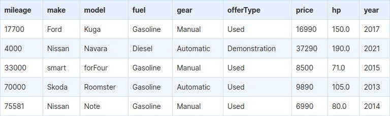
Here we can see several possible values for fields like fuel, gear, and offerType. We will print their unique values to understand how many are there and how to treat them. Presented below is the output for gear and offer type. There are many types of fuel that we will group later.
cars.gear.unique()
# ['Manual' 'Automatic' 'Semi-automatic']
cars.offerType.unique()
# ['Used' 'Demonstration' "Employee's car" 'Pre-registered' 'New']
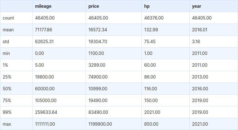
We will describe the fields containing numeric values. It will show descriptive statistics for each column, such as mean or standard deviation. A trick applies here to avoid scientific notation and show some cleaner output.
We can spot some outliers and probably some errors -like a car with 1 hp-, but we'll worry about them in a future post.
cars.describe(percentiles=[.01, .25, .5, .75, .99]).apply(
    lambda s: s.apply('{0:.2f}'.format))
Now we have a deeper understanding of what the data and columns contain. We can start with data visualization. We'll see now how makes distribute and then continue with price prediction.
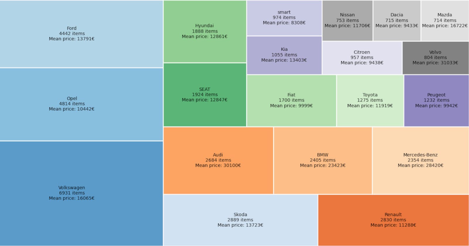
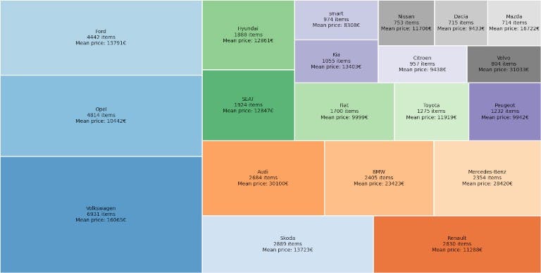
Visualizing Car Makes
To show the top 20 makes in the dataset, we will group them by value count. That means that we'll create a new data frame with just the makes and their counts, i.e., "Volkswagen 6931".
Then sort them and take the top 20. The last line will rename the columns for later manipulation.
makes = pd.DataFrame(cars.make.value_counts())
makes.reset_index(level=0, inplace=True)
makes = makes.sort_values(by='make', ascending=False).head(20)
makes.columns = ('make', 'size')
We will calculate the mean price per make to show along with the number of items.
First, group cars by make from the original dataset and extract their means into a new DataFrame. Also, reset the index.
Then, merge mean prices back into the makes DataFrame. It will now contain makes, size, and price columns.
group = cars.groupby(cars.make)
mean_price = pd.DataFrame(group.price.mean())
mean_price.reset_index(level=0, inplace=True)
makes = pd.merge(makes, mean_price, how='left', on='make')
The last step for this part is to show the graph. Two new imports are required to plot it.
We'll start by creating the labels that will show the make, numbers of items, and mean price.
Next, use squarify to divide in rectangles and size them according to the number of items. The essential parameters are sizes and label. The rest are purely cosmetic.
The last two lines are to hide the axis and show the plot. Depending on your environment, that final step might not be necessary.
import matplotlib.pyplot as plt
import squarify
labels = ["%s\n%d items\nMean price: %d€" % (label) for label in
    zip(makes['make'], makes['size'], makes['price'])]
squarify.plot(sizes=makes['size'], label=labels, alpha=.8,
    color=plt.cm.tab20c.colors, edgecolor="white", linewidth=2)
plt.axis('off')
plt.show()
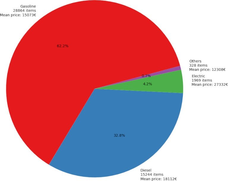
Visualizing Fuel Types
We will take a look at fuels now, but grouping the electrics and Others.
cars['fuel'] = cars['fuel'].replace(
    ['Electric/Gasoline', 'Electric/Diesel', 'Electric'],
    'Electric')
cars['fuel'] = cars['fuel'].replace(
    ['CNG', 'LPG', 'Others', '-/- (Fuel)', 'Ethanol', 'Hydrogen'],
    'Others')
And then calculate the totals similar to the previous case, but now plotting a pie chart.
This code block is longer but looks like the last one, so no need to explain a lot.
Summarized, create a new data frame with value counts, group by fuel, and extract means. Then, merge those two. Prepare the labels just as before and plot the pie chart.
fuels = pd.DataFrame(cars['fuel'].value_counts())
group = cars.groupby(cars['fuel'])
mean_price = pd.DataFrame(group.price.mean())
mean_price.reset_index(level=0, inplace=True)
fuels.reset_index(level=0, inplace=True)
fuels.columns = ('fuel', 'size')
fuels = pd.merge(fuels, mean_price, how='left', on='fuel')

labels = ["%s\n%d items\nMean price: %d€" % (label) for label in
    zip(fuels['fuel'], fuels['size'], fuels['price'])]
fig1, ax1 = plt.subplots()
ax1.pie(fuels['size'], labels=labels,
    autopct='%1.1f%%', startangle=15, colors=plt.cm.Set1.colors)
ax1.axis('equal')
plt.show()
Fuel types per Year
In this kind of exploratory analysis, sometimes we try things out or follow a hunch. In this case, we thought that electrics are getting trendy and diesel is on (a relative) decline.
To test that, we only need to create a countplot: count how many cars from each fuel type are on the dataset per year. We are going to show the results after the grouping we did in a previous step. That will avoid some noise and plot similar fuel types together (i.e., Electric and Electric/Gasoline).
We will use the seaborn library. With just year for the x-axis and fuel for the grouping, it will handle the rest autonomously.
import seaborn as sns

sns.countplot(x="year", hue="fuel", data=cars)
plt.show()
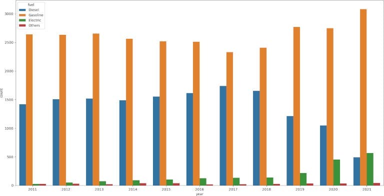
We were right, but that's not the essential point. It is that we proved our hypothesis in a few minutes with a simple graph.
What about the price?
You probably noticed that we didn't even mention which is perhaps the most relevant column: price. That's not a slip from our side. We will write a second part that will explain how price is related to other variables and compare different price prediction algorithms.
UPDATE: You can continue reading the second part .
Conclusion
As we've seen, importing CSV data into python pandas is relatively easy. It gets more complicated as we start to look for insights. Some simple functions like head or describe will give us much information.
With all that early knowledge, we can use graphs to visualize how the data is distributed and even how variables evolve - like fuel types. We can use that knowledge to form hypotheses and quickly prove or disprove them.
Originally published at https://www.zenrows.com