Car Price Prediction in Python

Web developer who has been working for several startups for more than 10 years, having worked with a wide variety of sectors and technologies. Engineer turned entrepreneur.
Last week, we did some Exploratory Data Analysis to a car dataset . After working with the dataset and gathering many insights, we'll focus on price prediction today.
The dataset comprises cars for sale in Germany , the registration year being between 2011 and 2021. So we can assume that it is an accurate representation of market price nowadays.
Prerequisites
For the code to work, you will need python3 installed . Some systems have it pre-installed. After that, install all the necessary libraries by running pip install.
# last week
pip install pandas matplotlib squarify seaborn
# new libs
pip install scipy sklearn catboost statsmodels
Data Cleaning
Let's say we want to predict car prices based on attributes. For that, we will train a model. Let's start by replacing registration year with age and removing make and model - we won't be using them for the predictions.
cars['age'] = datetime.now().year - cars['year']
cars = cars.drop('year', 1)
cars = cars.drop('make', 1)
cars = cars.drop('model', 1)
We talked about outliers last week, and now it's time to remove them. We'll do that by removing the items in which the z score for the price, horsepower, or mileage is higher than 3. In short, this means taking out the values that deviate more than three standard deviations from the mean.
Before that, dropna will remove all lines with empty or null values.
from scipy import stats

cars = cars.dropna()
cars = cars[stats.zscore(cars.price) < 3]
cars = cars[stats.zscore(cars.hp) < 3]
cars = cars[stats.zscore(cars.mileage) < 3]
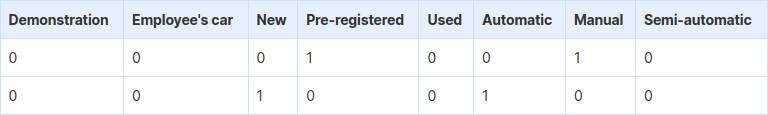
Next, we will replace the category values (offer type and gear) with boolean markers. In practice, this means creating new columns for each category type (i.e., for gear, it will be Automatic, Manual, and Semi-automatic).
There is a function in pandas to do that: get_dummies.
offerTypeDummies = pd.get_dummies(cars.offerType)
cars = cars.join(offerTypeDummies)
cars = cars.drop('offerType', 1)

gearDummies = pd.get_dummies(cars.gear)
cars = cars.join(gearDummies)
cars = cars.drop('gear', 1)
Checking Correlation Visually
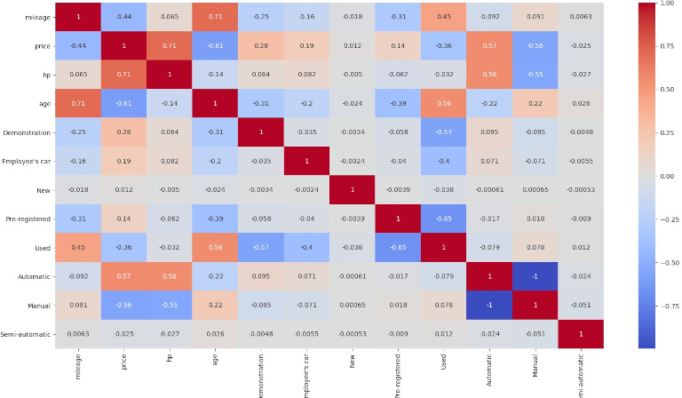
We are going to plot variable correlation using seaborn heatmap. It will show us graphically which variables are positively or negatively correlated.
The highest correlation shows for age with mileage - sounds fine - and price with horsepower - no big news either. And looking at negative correlation, price with age - which also seems natural.
We can ignore the relation between Manual and Automatic since it's evident that you will only have one or the other - there are almost no Semi-automatics.
import seaborn as sns

sns.heatmap(cars.corr(), annot=True, cmap='coolwarm')
plt.show()
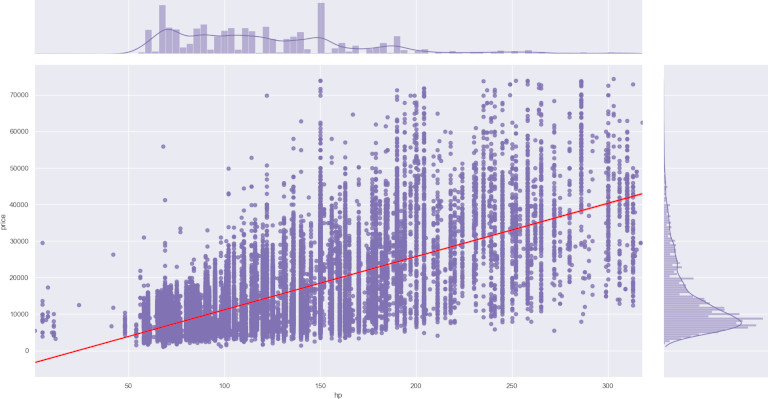
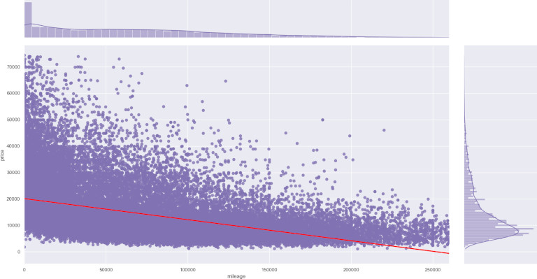
For a double check, we are going to plot horsepower and mileage variables with the price. We'll do it with seaborn jointplot.
It will plot all the entries and a line for the regression. For brevity, there is only one code snippet. The second one would be the same, replacing hp with mileage.
sns.set_theme(style="darkgrid")
sns.jointplot(x="hp", y="price", data=cars,
    kind="reg", color="m", line_kws={'color': 'red'})
plt.show()
Price Prediction
We are reaching the critical part. We will try three different prediction models and see which one performs better.
We need two variables, Y and X, containing price and all the remaining columns. We will use these new variables for the other models too. Then, we split the data for training and testing in a 70%-30% distribution.
Disclaimer: we did several tests with all the models and chose the best results for each model. Not the same vars apply, and some "magic" numbers will appear. We adjusted those mainly through trial and error.
from sklearn.model_selection import train_test_split

X = cars.drop('price', 1)
Y = cars.price
X_train, X_test, y_train, y_test = train_test_split(
    X, Y, train_size=0.7, test_size=0.3, random_state=100)
linear_model from sklearn
To train the first LinearRegression model, we will pass the train data to the fit method and then the test data to predict.
To check the results, we'll be using R-squared for all of them. In this case, the result is 0.81237.
from sklearn import linear_model
from sklearn.metrics import r2_score

lm = linear_model.LinearRegression()
lm.fit(X_train, y_train)
y_pred = lm.predict(X_test)
print(r2_score(y_true=y_test, y_pred=y_pred)) # 0.81237
Regressor from CatBoost
Next, we'll use Regressor from CatBoost. The model's created with some numbers that we adjusted by testing. Similar to the previous one, fit the model with the train data and check the score, resulting in 0.92416.
There is a big difference since this method is much slower, more than 20 seconds. It might be a closer match, but not a good option if it must run instantly.
from catboost import CatBoostRegressor

model = CatBoostRegressor(iterations=6542, learning_rate=0.03)
model.fit(
    X_train, y_train,
    eval_set=(X_test, y_test),
)
print(model.score(X, Y)) # 0.92416
OLS from statsmodels
For statsmodels, we will change X's value and take only mileage, hp, and age. The difference is almost 10% better than with the previous values.
R-squared is 0.91823, and it runs in under two seconds - counting the data load.
import statsmodels.api as sm

X = cars[['mileage', 'hp', 'age']]

model = sm.OLS(Y, X).fit()
predictions = model.predict(X)
print(model.rsquared) # 0.91823
Extra Ball: Best Prediction
What happens if we do not drop make and model? Two of the models would perform worse, but not CatBoost. It will take much longer and use more space. We would have more than 700 feature columns. But it is worth it if you are after accuracy.
For brevity, we will not reproduce all the manipulations we did previously. Instead of dropping make and model, create dummies for them and then continue as before.
makeDummies = pd.get_dummies(cars.make)
cars = cars.join(makeDummies)
cars = cars.drop('make', 1)

modelDummies = pd.get_dummies(cars.model)
cars = cars.join(modelDummies)
cars = cars.drop('model', 1)

# the rest of the features, just as before
# split train and test data

model = CatBoostRegressor(iterations=6542, learning_rate=0.03)
model.fit(
    X_train, y_train,
    eval_set=(X_test, y_test),
)
print(model.score(X, Y)) # 0.9664
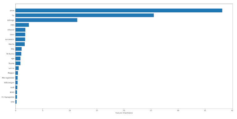
This model exposes a method to obtain feature importance. We can use that data with a bar chart to check which features affect the prediction the most. We will limit them to 20, but as you'll see, two of them - excluding price itself - carry all the weight.
Age not being significant might look suspicious at first glance. But it makes sense. As we saw in the correlation graph, age and mileage go hand in hand. So there is no need for the two of them to carry all the weight.
sorted_feature_importance = model.get_feature_importance().argsort(
    )[-20:]
plt.barh(
    cars.columns[sorted_feature_importance],
    model.feature_importances_[sorted_feature_importance]
)
plt.xlabel("Feature Importance")
plt.show()
Estimate Car Price
Let's say that you want to buy or sell your car. You collect the features we provide (mileage, year, etcetera). How to use the prediction model for that?
We'll choose CatBoost again and use their predict method for that. We would need to go all the way again by transforming all the data with dummies, so we'll summarize. This process would be extracted and performed equally for training, test, or actual data in a real-world app.
We will also need to add all the empty features (i.e., all the other makes) that the model supports.
Here we present an example with three cars for sale. We manually entered all the initial features (price included), so we can compare the output. As you'll see, the predictions are not far from the actual price.
realData = pd.DataFrame.from_records([
    {'mileage': 87000, 'make': 'Volkswagen', 'model': 'Gold',
        'fuel': 'Gasoline', 'gear': 'Manual', 'offerType': 'Used',
        'price': 12990, 'hp': 125, 'year': 2015},
    {'mileage': 230000, 'make': 'Opel', 'model': 'Zafira Tourer',
        'fuel': 'CNG', 'gear': 'Manual', 'offerType': 'Used',
        'price': 5200, 'hp': 150, 'year': 2012},
    {'mileage': 5, 'make': 'Mazda', 'model': '3', 'hp': 122,
        'gear': 'Manual', 'offerType': 'Employee\'s car',
        'fuel': 'Gasoline', 'price': 20900, 'year': 2020}
])

realData = realData.drop('price', 1)
realData['age'] = datetime.now().year - realData['year']
realData = realData.drop('year', 1)

# all the other transformations and dummies go here

fitModel = pd.DataFrame(columns=cars.columns)
fitModel = fitModel.append(realData, ignore_index=True)
fitModel = fitModel.fillna(0)

preds = model.predict(fitModel)
print(preds) # [12213.35324984 5213.058479 20674.08838559]
Conclusion
As a quick note on the three models, sklearn performs a bit worse. And the other two are pretty similar in results - if excluding makes and models - but not on time spent training. So it might be a crucial aspect to consider when choosing between them.
If you are after high accuracy, train the CatBoost model with all the available data. It might take up to a minute, but it can be stored in a file and instantly loaded when needed.
As you've seen, loading a ZenRows generated dataset into pandas is quite simple. Then, there are some steps to perform: describe, explore manually, look at the values, check for empty or nulls.
These are everyday tasks when first testing a dataset. From there, standard practices such as generating dummies or removing outliers. And then the juicy part. In this case, price prediction using linear regression, but it could be anything.
Originally published at https://www.zenrows.com


